How fast can cheap LLMs query ClickHouse?
Comparing cheap models on SQL accuracy, response time and cost, then using one to query wildlife and ship data.
- clickhouse
- llm
- benchmark
- data-exploration
My previous benchmark of 22 models tested whether LLMs could write ClickHouse SQL. This time I wanted to know how quickly a cheap model could turn a question into a database result, and what each request would cost.
In this run, DeepSeek V4.1 Flash returned a correct answer in 88% of attempts. The median wait from sending the question to receiving the database result was 672 ms. Model charges came to about four US cents per 1,000 attempts, with input caching.
Latency matters because one answer often leads to the next question. Fast, inexpensive replies could make that sequence a more practical way to explore data: ask, inspect a chart, narrow the question and ask again. I tried it in a small prototype using the same model.
The benchmark: correctness, delay and cost
The October 7, 2026 run used 60 questions, five repetitions and five models: 1,500 attempts against a synthetic ClickHouse database with one million events and 10,000 users. I ran the generated SQL and compared the returned data with reference results checked before the test. Each attempt had one model call, with no retries or SQL repairs.
| Model | Correct | Median | p95 | USD / 1,000 |
|---|---|---|---|---|
| DeepSeek V4.1 Flash | 88.0% | 0.672 s | 1.847 s | $0.041 |
| GPT-6 Luna | 79.0% | 1.202 s | 2.175 s | $0.151 |
| Solar Mini 4 | 64.3% | 3.106 s | 7.776 s | $0.039 |
| Mercury 2.5 | 59.0% | 0.792 s | 1.456 s | Unknown |
| Granite 4.2 8B | 58.7% | 0.909 s | 1.704 s | $0.041 |
The timer starts when the request goes to OpenRouter and stops when the ClickHouse result has arrived and been parsed. It covers the complete SQL response, query execution and returned rows. The p95 column shows the time within which 95% of completed results arrived.
The timing columns include wrong answers that executed successfully. Errors and timeouts count as failures when calculating accuracy and the share of correct answers delivered on time. Mercury had 39 rate-limit failures and six timeouts, with incomplete billing. Every model used a fixed provider through OpenRouter with reasoning disabled. Luna used OpenAI’s priority service.
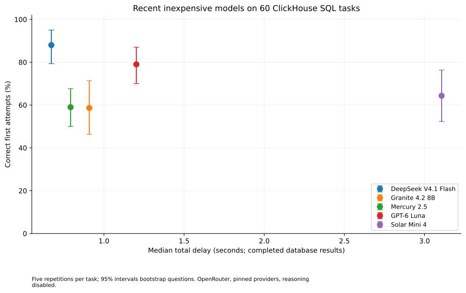
The bars show 95% confidence intervals. These are based on the sixty questions, keeping each question’s five attempts together. Open the full-size figure.
The costs reflect this repeated set of requests. For DeepSeek, 82.9% of input tokens came from the prompt cache. Pricing those tokens without the cache discount gives an estimate of $0.083 per 1,000 attempts. Solar’s price included a promotion. Hosting is excluded. The full results and methodology record the prices and settings used for this run.
I selected models announced or released in the two months before the run. I could not test Mistral Large 4 or Qwen3.8 Flash because the account’s privacy settings blocked their available providers. The test data and required outputs differ from the previous article, so the accuracy scores cannot be compared directly.
Which questions worked?
The questions were split into six difficulty levels. DeepSeek answered all thirty questions in the first three levels correctly on all five repeats: 150/150 attempts. These cover filtering, aggregation and simpler ClickHouse operations. On the hardest ten questions, it passed 25/50 attempts.
Granite, an 8B model, passed all fifty attempts at the first level, then 35/50 at the second and 17/50 at the third. DeepSeek V4.1 Flash is a much larger model that uses only part of its network for each token. The stronger result here came from a large model with a low API price.
Some failures were easy to miss without checking the data. In a retention question, DeepSeek counted each day’s users separately instead of following the group from the first day. The SQL ran but answered a different question. Another query passed a DateTime64 value to windowFunnel and failed on the tested ClickHouse version.
The provider affects response time
A second study ran another 1,500 attempts, switching between five DeepSeek provider and precision combinations, one request at a time. It included an older V4 Flash baseline alongside V4.1 Flash. Two of the V4.1 combinations returned these results:
| Route | Correct | Median | p95 | USD / 1,000 |
|---|---|---|---|---|
| InferenceNet FP8 | 88.7% | 0.800 s | 1.823 s | $0.043 |
| Sail Research FP4 | 90.7% | 1.716 s | 3.743 s | $0.028 |
The study’s rule favored cost once accuracy and five-second response targets were met; Sail won. For the prototype, I chose InferenceNet because 85.3% of attempts returned a correct result within two seconds, compared with 60.0% for Sail. The extra cost was about $0.015 per 1,000 attempts. Sail’s accuracy was two percentage points higher, but the 95% confidence interval for the difference ran from −1 to +6 points.
FP8 and FP4 are the eight-bit and four-bit formats reported by the providers. Different providers ran the two formats, so this test cannot tell us how much of the difference came from quantization alone. Cache discounts also affect the bill. The provider comparison has the full details.
The prototype uses deepseek/deepseek-v4.1-flash on inference-net/fp8, with FP8 required, fallback disabled and reasoning disabled. The gateway handles one model request at a time. The reported timings are for one user.
From a question to executed SQL
The application sends the model a question, the table definitions and the information needed to interpret the columns. The model writes SQL. The application checks the query, runs it with restricted database credentials and returns the rows.
The benchmark prompt includes column types, the ClickHouse version, the UTC time zone, the available dates and values such as event types. It asks for one SELECT, without an explanation or FORMAT clause. Each question also specifies the columns, order and limits expected in the answer.
For example, one recorded question was:
Show the number of events per day in January 2024. Output contract: return only these columns, in this order: day as Date, event count. Order/limit: day ascending.
DeepSeek generated this query on the first run:
SELECT toDate(timestamp) AS day, count() AS event_count
FROM events
WHERE timestamp >= '2024-01-01 00:00:00'
  AND timestamp < '2024-02-01 00:00:00'
GROUP BY day
ORDER BY day ASC
It returned 31 rows matching the reference. The model received the schema and question; ClickHouse read the events and counted them by day. Using February 1 as the exclusive end includes all of January, whatever the timestamp precision.
The benchmark script calls ClickHouse’s HTTP API directly and adds FORMAT JSONCompact itself. It uses a read-only account, two query threads, a 2 GB memory limit, a ten-second execution limit and limits on the rows and bytes returned. The query cache is disabled. Earlier reference and trial runs had already read the data, so storage caches were warm. The timer stops before scoring the answer.
For the prototype, I used the official ClickHouse MCP server, which provides a run_query tool. Once the MCP client is connected and authenticated, the call is:
result = await MCP.call_tool("run_query", {"query": sql})A Python/FastAPI backend sends the question through a gateway to OpenRouter. The model returns SQL, a chart type and the columns to use in a paint_canvas tool call. The backend checks the response and sends the SQL to ClickHouse through MCP.
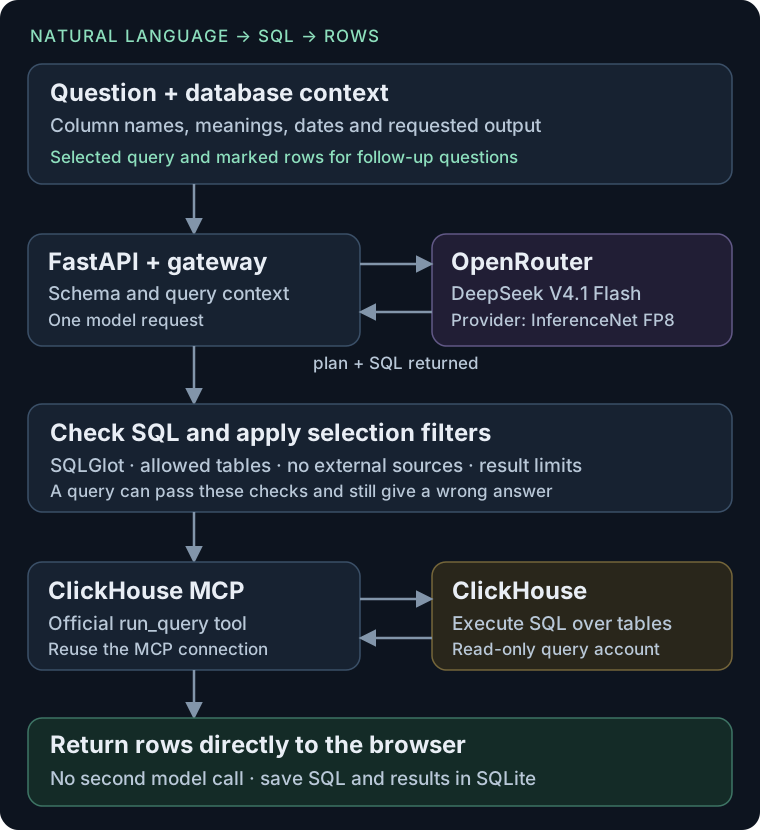
SQLGlot checks the query’s structure before execution. The backend accepts one read query using only tables from the selected dataset. It rejects writes, external table functions, model-supplied query settings and output destinations. The ClickHouse account enforces its own read-only permissions and resource limits.
For a follow-up such as “show photographs from this cell”, the application uses the saved SQL and selected result row to recover the original species, date and geographic filters. It applies those filters to the new query. Existing views supply their SQL, column names and a two-row sample to the model. The full dataset stays in ClickHouse.
The browser draws the returned rows without asking the model to write a summary first. It uses Plotly for charts, Leaflet for maps and tracks, SVG for seasonal wheels and Canvas2D for surfaces that can be rotated. SQLite keeps the SQL and results. LibreChat supplies login; FastAPI handles the queries.
Trying it on wildlife and ship data
I tried the same loop in an interface with chat on the right and a canvas on the left. A question creates a view. From there, I can ask for a comparison, select part of a chart and inspect the records behind it.
I loaded 282.9 million wildlife observations from the iNaturalist open dataset, and 109.3 million ship position reports from NOAA, with IBTrACS storm tracks. The ship data covers Gulf and Florida waters from September 15 through October 15, 2024. Wildlife photographs load on demand, with license and photographer credits.
In the first example, I ask for a map of monarch observation density in 2025, add a seasonal view and then a heatmap of month against latitude. I select August at 40–45° north, switch to a 3D surface and ask for photographs from that cell. The last query lets me inspect the observations behind that part of the chart.
The 87-second recording runs at original speed, including model and database waits. A script types the prepared prompts and clicks the controls. The queries ran during the recording.

An 18-second excerpt at original speed, with the chat sidebar cropped. The full video retains the prompts. Enlarged photograph: © Sheila S, CC-BY. All photograph credits.
For a selected heatmap, “make it 3d” changes the view using the same rows. It makes no model call and runs no SQL. Rotation and playback also use loaded data. A new question about the records goes through the query loop again.
The other examples compare fungal seasons between hemispheres, examine moving and nearly stationary Mississippi vessels, and replay the cargo ship ELSA alongside Hurricane Milton. The ELSA example then compares daily vessel counts around Tampa Bay and Port Everglades with each area’s early-October baseline:
The full recording lasts 2 minutes 11 seconds, including the longer waits. Playback estimates positions between nearby historical reports and leaves long gaps blank. Optional NASA GIBS imagery shows the selected day, rather than each playback timestamp.
Timing the complete interactions
The prototype sends more context than the benchmark and asks for chart instructions as well as SQL. The four completed demo runs used 17 model requests, with a 2.35-second median wait for data and $0.00843 in model charges:
| Sequence | Calls | Time to data | USD |
|---|---|---|---|
| Monarch year | 4 | 1.75–3.23 s | $0.00172 |
| Fungal seasons | 4 | 1.87–2.35 s | $0.00194 |
| Mississippi ships | 4 | 2.01–4.11 s | $0.00205 |
| ELSA and Milton | 5 | 5.75–16.62 s | $0.00273 |
The slowest request spent 15.43 seconds waiting for the model and 0.72 seconds in the query tool. Across the four runs, the tool took 28–722 ms, including MCP transport and result processing. Four chart changes that reused loaded data were measured as ready by the browser in 138–257 ms, without inference.
These timings stop when the browser has the result data. Animations and photograph loading can continue afterward. The demos use prepared prompts; they do not measure accuracy on new questions.
The longer ELSA waits interrupt the flow of questions. Even the shorter waits of roughly two seconds are noticeable when each result suggests something else to look at. Faster replies would make it easier to follow those questions while keeping the previous result in mind.
The SQL still needs checking
The saved demos passed 76 automated checks, including comparisons with independent reference queries. Earlier attempts had errors. One photo query returned 773 rows because it limited each species to twelve photos instead of limiting the whole result. A date filter left out the final day, and a speed query failed because it grouped by an aggregate alias. The saved runs include the failed attempts; the runbook gives the successful prompts.
The meaning of the data needs care too. Wildlife counts measure reported observations. The coastal activity charts count ships sending position reports inside each map area. A long period at low speed does not show why a ship was there. The prototype leaves earlier results intact after a failed query and waits for another request; it does not repair the SQL automatically.
Code and measurements
The public code and measurements contain the saved benchmark requests, SQL, results, scoring code, data loaders and prototype. The benchmark directory explains how to check the saved results without making new model calls.
The benchmark suggests that cheap models can already handle many ordinary data questions, while complex queries still need closer checking. Low cost makes repeated requests affordable. Low latency could make those requests a routine way to explore: see a result, follow a question it raises and keep going.