ClickHouse Compression Codecs for Time-Series Data: A Benchmark
Five ClickHouse codec configurations benchmarked on 100M rows of time-series data: storage, query latency and ingest throughput, with a decision tree for codec selection.
- clickhouse
- compression
- time-series
- benchmark
TLDR
- On 100M synthetic time-series rows, per-column codecs with ZSTD(3) achieved 4.23× compression, versus 1.67× for default LZ4.
- LZ4 was usually faster for warm queries and ingest. ZSTD(9) gave no meaningful storage gain over ZSTD(3) and cut ingest throughput by 28%.
- Choose codecs by column and workload: regular timestamps and counters compressed especially well; Gorilla could expand noisy floats. The dataset fit in RAM.
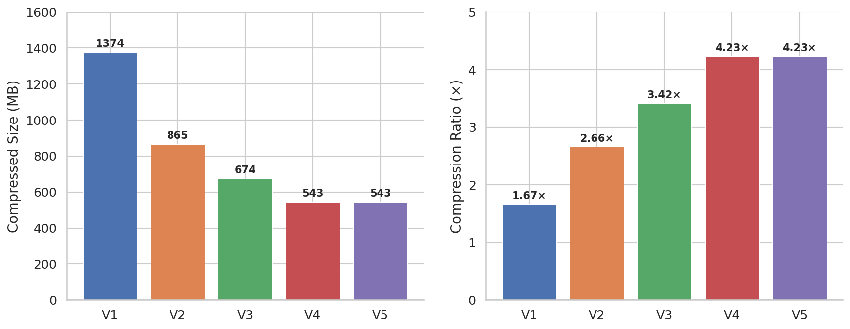
I benchmarked five compression codec setups on 100 million rows of synthetic time-series data in ClickHouse 25.11, from plain default LZ4 to per-column codecs (DoubleDelta, Delta, Gorilla) combined with ZSTD. I measured three things: storage size, query latency (cold and warm), and ingest speed.
All data, scripts and plots are in comino/blog-experiments. Numbers below are median ± IQR over 10 runs.
Setup
- Server: Hetzner CX53 with 16 vCPU (AMD EPYC), 32 GB RAM, NVMe SSD
- ClickHouse: 25.11.3.54, default settings
- Dataset: 100M rows × 6 columns, simulating Prometheus-style metrics
- Cold runs: all ClickHouse and OS caches dropped before each measurement
- Warm runs: one warmup query first, then 10 measured runs
One caveat up front: the whole dataset fits in RAM (543 MB to 1.37 GB depending on codec). So my “cold” numbers show NVMe re-read plus decompression, not the sustained disk I/O you would see when data is much bigger than memory. More on that below.
Data Generation
The 100M rows come from ClickHouse’s numbers() function:
INSERT INTO exp01_compression.source
SELECT
    toDateTime('2024-01-01 00:00:00') + intDiv(number, 50) AS timestamp,
    ['cpu_usage','disk_io','http_requests_total','mem_free','net_bytes_sent']
        [1 + (number % 5)] AS metric_name,
    50 + 30 * sin(number / 1000.0) + (rand(number) % 1000) / 2000.0 AS value,
    concat('host-', toString(number % 50)) AS host,
    ['us-east','us-west','eu-central','ap-south'][1 + (rand(number + 1) % 4)] AS region,
    intDiv(number, 50) AS counter
FROM numbers(100000000);
That gives me:
timestamp: strict 1-second intervals, ~115 days of datacounter: strictly increasing UInt64value: a sine wave plus noise, like a noisy gauge metricmetric_name,host,region: LowCardinality strings (5, 50 and 4 distinct values)
All tables use ORDER BY (metric_name, host, timestamp). After insert, OPTIMIZE TABLE … FINAL merged everything into a single part.
This data is ideal for compression: perfectly regular timestamps, perfectly monotone counters. Real data is messier and will compress less. Keep that in mind for every ratio below.
The Five Variants
-- V1: Default (LZ4)
CREATE TABLE v1_default (
    timestamp DateTime,
    metric_name LowCardinality(String),
    value Float64,
    host LowCardinality(String),
    region LowCardinality(String),
    counter UInt64
) ENGINE = MergeTree()
ORDER BY (metric_name, host, timestamp);

-- V2: ZSTD(3) on all columns
CREATE TABLE v2_zstd (
    timestamp DateTime CODEC(ZSTD(3)),
    metric_name LowCardinality(String) CODEC(ZSTD(3)),
    value Float64 CODEC(ZSTD(3)),
    host LowCardinality(String) CODEC(ZSTD(3)),
    region LowCardinality(String) CODEC(ZSTD(3)),
    counter UInt64 CODEC(ZSTD(3))
) ENGINE = MergeTree()
ORDER BY (metric_name, host, timestamp);

-- V3: Per-column specialized + LZ4
CREATE TABLE v3_percolumn (
    timestamp DateTime CODEC(DoubleDelta, LZ4),
    metric_name LowCardinality(String) CODEC(LZ4),
    value Float64 CODEC(Gorilla(8), LZ4),
    host LowCardinality(String) CODEC(LZ4),
    region LowCardinality(String) CODEC(LZ4),
    counter UInt64 CODEC(Delta(8), LZ4)
) ENGINE = MergeTree()
ORDER BY (metric_name, host, timestamp);

-- V4: Per-column specialized + ZSTD(3)
CREATE TABLE v4_percolumn_zstd (
    timestamp DateTime CODEC(DoubleDelta, ZSTD(3)),
    metric_name LowCardinality(String) CODEC(ZSTD(3)),
    value Float64 CODEC(Gorilla(8), ZSTD(3)),
    host LowCardinality(String) CODEC(ZSTD(3)),
    region LowCardinality(String) CODEC(ZSTD(3)),
    counter UInt64 CODEC(Delta(8), ZSTD(3))
) ENGINE = MergeTree()
ORDER BY (metric_name, host, timestamp);

-- V5: Same as V4, but ZSTD(9) on most columns
CREATE TABLE v5_aggressive (
    timestamp DateTime CODEC(DoubleDelta, ZSTD(9)),
    metric_name LowCardinality(String) CODEC(ZSTD(9)),
    value Float64 CODEC(Gorilla(8), ZSTD(3)),
    host LowCardinality(String) CODEC(ZSTD(9)),
    region LowCardinality(String) CODEC(ZSTD(9)),
    counter UInt64 CODEC(Delta(8), ZSTD(9))
) ENGINE = MergeTree()
ORDER BY (metric_name, host, timestamp);
The (8) in Gorilla(8) and Delta(8) is the value width in bytes (Float64/UInt64 = 8). In V5, value stays on ZSTD(3): the Gorilla output of noisy floats is basically incompressible, so a higher ZSTD level has nothing to work with.
Storage
Sizes come from system.parts_columns (column data only, one merged part per table):
| Variant | Compressed | Uncompressed | Ratio |
|---|---|---|---|
| V1 (LZ4 default) | 1,374.5 MB | 2,300.9 MB | 1.67× |
| V2 (ZSTD all) | 864.7 MB | 2,301.1 MB | 2.66× |
| V3 (per-col + LZ4) | 673.6 MB | 2,301.1 MB | 3.42× |
| V4 (per-col + ZSTD) | 543.4 MB | 2,301.1 MB | 4.23× |
| V5 (aggressive) | 543.4 MB | 2,301.1 MB | 4.23× |
V4 and V5 differ by 141 KB on 543 MB. The specialized pre-codecs do the heavy lifting; raising ZSTD from level 3 to 9 buys nothing here.
Where the difference comes from, per column:
| Column | Type | V1 | V3 | V4 | V1 Ratio | V3 Ratio | V4 Ratio |
|---|---|---|---|---|---|---|---|
| timestamp | DateTime | 401.7 MB | 477 KB | 459 KB | 1.00× | 839× | 872× |
| counter | UInt64 | 420.1 MB | 977 KB | 949 KB | 1.90× | 818× | 843× |
| value | Float64 | 551.2 MB | 634.5 MB | 541.7 MB | 1.45× | 1.26× | 1.48× |
| metric_name | LC(String) | 482 KB | 470 KB | 111 KB | 208× | 213× | 908× |
| host | LC(String) | 484 KB | 471 KB | 112 KB | 207× | 213× | 898× |
| region | LC(String) | 486 KB | 473 KB | 116 KB | 206× | 212× | 867× |
Why 872× on timestamps? The data is sorted, so within each (metric_name, host) group the timestamps step by exactly 1 second. DoubleDelta turns that into near-constant zeros, and ZSTD squeezes those to almost nothing. Plain LZ4 without a pre-codec gets 1.0×: it simply cannot see the pattern. Same story for the counter column with Delta.
Why does value barely compress? It’s a sine wave plus random noise. Noise has no pattern to exploit. Worse: V3 (Gorilla+LZ4) lands at 1.26×, below plain LZ4’s 1.45×. Gorilla’s XOR encoding actually expanded the noisy data.
When Gorilla Helps
Gorilla XORs each value with the previous one and stores only the changed bits. Nearly-identical neighbors compress great; noisy neighbors change all the bits and add overhead. I tested four distributions on 10M-row tables:
| Distribution | Description | LZ4 Ratio | Gorilla+LZ4 Ratio |
|---|---|---|---|
| Monotone | f(t) = t × 0.001 | 1.74× | 44.7× |
| Spiky | 99% zeros, 1% spikes | 1.62× | 30.8× |
| Sinus + noise | smooth + noise | 1.31× | 2.48× |
| Random | uniform random | 1.05× | 1.29× |
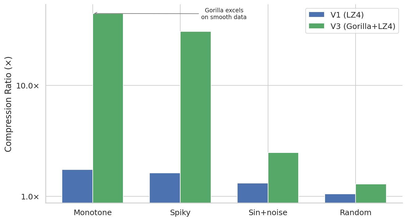
Rule of thumb:
- ✅ Slowly drifting values: battery levels, temperatures, counters stored as floats
- ✅ Sparse data that is mostly zeros
- ❌ Noisy gauges: CPU%, latency, throughput
- ❌ Random values
Query Performance
I ran 10 queries covering common access patterns:
-- Q1: Point lookup (1 host, 1 hour)
SELECT avg(value) FROM {table}
WHERE metric_name='cpu_usage' AND host='host-0'
  AND timestamp BETWEEN '2024-01-01 00:00:00' AND '2024-01-01 01:00:00';

-- Q2: Range scan (1 metric, 7 days)
SELECT avg(value) FROM {table}
WHERE metric_name='cpu_usage'
  AND timestamp BETWEEN '2024-01-01' AND '2024-01-08';

-- Q3: Top-K GROUP BY host
SELECT host, count(), avg(value) FROM {table}
WHERE metric_name='cpu_usage'
GROUP BY host ORDER BY count() DESC LIMIT 10;

-- Q4: Point lookup (1 host, 1 hour, multi-agg)
SELECT avg(value), min(value), max(value) FROM {table}
WHERE metric_name='cpu_usage' AND host='host-3'
  AND timestamp BETWEEN '2024-01-05 12:00:00' AND '2024-01-05 13:00:00';

-- Q5: Full table scan, touches the value column
SELECT count() FROM {table} WHERE value > 60;

-- Q6: Heavy aggregation, reads all columns
SELECT metric_name, host, avg(value), sum(counter) FROM {table}
GROUP BY metric_name, host ORDER BY avg(value) DESC LIMIT 20;

-- Q7: p99 percentile on value
SELECT metric_name, quantile(0.99)(value) AS p99 FROM {table}
GROUP BY metric_name;

-- Q8: Distinct counts on string columns
SELECT uniqExact(metric_name), uniqExact(host) FROM {table};

-- Q9: Last value per host (argMax)
SELECT host, argMax(value, timestamp) AS last_value FROM {table}
WHERE metric_name='cpu_usage' GROUP BY host;

-- Q10: Moving average (window function)
SELECT timestamp, avg(value) OVER (ORDER BY timestamp
  ROWS BETWEEN 59 PRECEDING AND CURRENT ROW) AS ma60
FROM {table}
WHERE metric_name='cpu_usage' AND host='host-0'
  AND timestamp BETWEEN '2024-01-01' AND '2024-01-02'
ORDER BY timestamp;
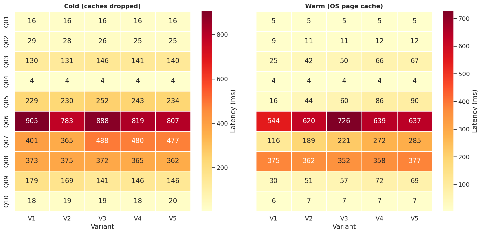
Cold (median ± IQR, ms, n=10)
| Query | Pattern | V1 LZ4 | V2 ZSTD | V3 per-col+LZ4 | V4 per-col+ZSTD | V5 aggressive |
|---|---|---|---|---|---|---|
| Q01 | Point lookup | 16 ± 1 | 16 ± 1 | 16 ± 0 | 16 ± 2 | 16 ± 2 |
| Q02 | Range 7d | 29 ± 3 | 28 ± 2 | 26 ± 1 | 25 ± 1 | 25 ± 2 |
| Q03 | Top-K hosts | 130 ± 14 | 131 ± 6 | 146 ± 3 | 141 ± 12 | 140 ± 10 |
| Q04 | Point lookup | 4 ± 1 | 4 ± 1 | 4 ± 1 | 4 ± 0 | 4 ± 1 |
| Q05 | Full scan WHERE | 229 ± 4 | 230 ± 16 | 252 ± 11 | 243 ± 12 | 234 ± 13 |
| Q06 | Multi-col agg | 905 ± 37 | 783 ± 18 | 888 ± 23 | 819 ± 9 | 807 ± 33 |
| Q07 | Percentile p99 | 401 ± 42 | 365 ± 10 | 488 ± 21 | 480 ± 28 | 477 ± 11 |
| Q08 | Distinct count | 373 ± 17 | 375 ± 24 | 372 ± 20 | 365 ± 21 | 362 ± 26 |
| Q09 | argMax | 179 ± 5 | 169 ± 5 | 141 ± 7 | 146 ± 7 | 146 ± 7 |
| Q10 | Window func | 18 ± 1 | 19 ± 1 | 19 ± 2 | 18 ± 1 | 20 ± 1 |
Warm (median ± IQR, ms, n=10)
| Query | Pattern | V1 LZ4 | V2 ZSTD | V3 per-col+LZ4 | V4 per-col+ZSTD | V5 aggressive |
|---|---|---|---|---|---|---|
| Q01 | Point lookup | 5 ± 0 | 5 ± 0 | 5 ± 1 | 5 ± 1 | 5 ± 1 |
| Q02 | Range 7d | 9 ± 0 | 11 ± 0 | 11 ± 1 | 12 ± 0 | 12 ± 1 |
| Q03 | Top-K hosts | 25 ± 0 | 42 ± 1 | 50 ± 1 | 66 ± 2 | 67 ± 6 |
| Q04 | Point lookup | 4 ± 1 | 4 ± 0 | 4 ± 0 | 4 ± 0 | 4 ± 0 |
| Q05 | Full scan WHERE | 16 ± 0 | 44 ± 3 | 60 ± 4 | 86 ± 5 | 90 ± 4 |
| Q06 | Multi-col agg | 544 ± 43 | 620 ± 37 | 726 ± 37 | 639 ± 31 | 637 ± 34 |
| Q07 | Percentile p99 | 116 ± 5 | 189 ± 19 | 221 ± 8 | 272 ± 12 | 285 ± 13 |
| Q08 | Distinct count | 375 ± 28 | 362 ± 24 | 352 ± 21 | 358 ± 32 | 377 ± 29 |
| Q09 | argMax | 30 ± 2 | 51 ± 2 | 57 ± 2 | 72 ± 5 | 69 ± 7 |
| Q10 | Window func | 6 ± 1 | 7 ± 0 | 7 ± 0 | 7 ± 0 | 7 ± 1 |
What the numbers say
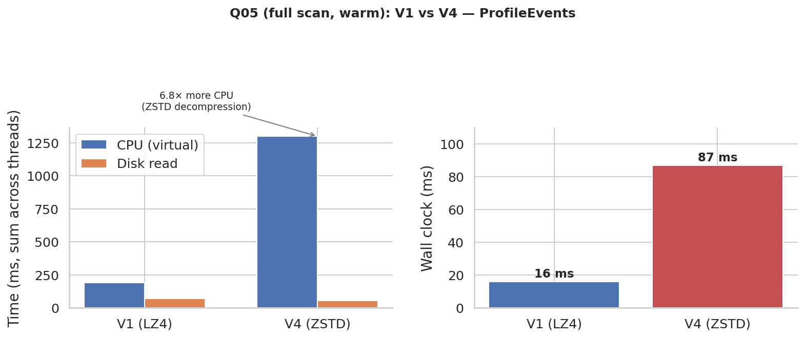
Warm queries: LZ4 wins almost everywhere. Look at Q05: V1 drops from 229 ms cold to 16 ms warm. V4 only drops from 243 ms to 86 ms. Once data sits in the page cache, V1 pays almost nothing for decompression, while V4 pays the ZSTD CPU cost on every single read. That cost doesn’t go away with caching.
Cold queries: compression helps where it actually compressed something. Q06 reads the counter column, which is 420 MB in V1 but under 1 MB in V4. Less data to read, faster cold query (819 ms vs 905 ms). Q09 benefits the same way from the tiny timestamp column.
Queries on the noisy value column: LZ4 wins, cold and warm. Q07 scans value, which is roughly the same size in every variant. Same bytes to read, but ZSTD is about 3× more expensive to decompress than LZ4. V1: 401 ms cold. V4: 480 ms.
Tiny queries don’t care. Point lookups (Q01, Q04, Q10) read a few granules; all variants are identical.
To check the “ZSTD costs CPU” explanation, I pulled ProfileEvents from system.query_log for warm Q05: both variants read the same 320 MB and 40M rows, disk time is nearly identical, but V4 burns 6.8× more CPU than V1 (1.3s vs 0.19s summed across threads). That’s the decompression. I only profiled this one query; the pattern is plausible for the other value-heavy queries but I did not verify each one.
A note on “cold” here: the dataset fits in RAM and the NVMe is fast, so cold vs warm mostly measures re-read overhead, not real disk pressure. On a system where data is much bigger than RAM, V4’s 2.5× smaller footprint would matter much more than it does in my numbers. My results understate the cold-query benefit of good compression.
Ingest
Single-threaded INSERT from a source table, three batch sizes, 10 runs each (median rows/s ± IQR):
| Variant | 10K batch | 100K batch | 1M batch |
|---|---|---|---|
| V1 (LZ4) | 147K ± 8K | 1,250K ± 31K | 5,666K ± 290K |
| V2 (ZSTD) | 144K ± 10K | 1,205K ± 148K | 4,651K ± 152K |
| V3 (per-col LZ4) | 147K ± 4K | 1,220K ± 98K | 4,808K ± 396K |
| V4 (per-col ZSTD) | 141K ± 23K | 1,198K ± 87K | 4,963K ± 333K |
| V5 (aggressive) | 137K ± 12K | 1,130K ± 51K | 3,559K ± 341K |
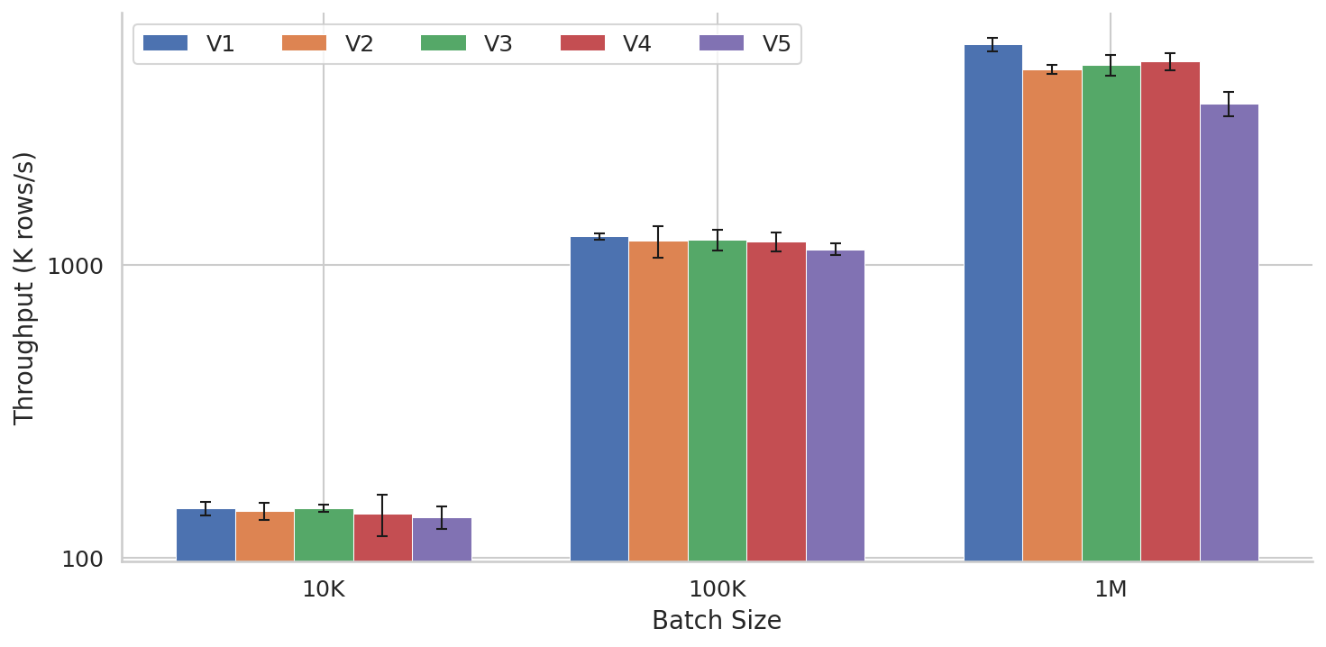
At small batches, per-INSERT overhead dominates and all variants look the same. At 1M-row batches:
- V1: 5.67M rows/s, fastest
- V4: 4.96M rows/s, 12% slower. The pre-codecs (Delta, DoubleDelta) are cheap.
- V5: 3.56M rows/s, 28% slower than V4 for zero compression gain. Clear lose-lose.
So Which One?
There is no single winner. Pick by workload:
| Your Workload | Best Choice | Why |
|---|---|---|
| Storage-constrained (cloud, cost per GB matters) | V4 | 2.5× smaller than V1 |
| Cold-query-heavy (data exceeds RAM) | V4 | Fewer disk reads beat decompression cost |
| Ingest-heavy (writes matter most) | V1 | Fastest ingest, minimal CPU |
| Warm-query-heavy (dashboards, data in RAM) | V1 | LZ4 is nearly free when cached |
| Don’t want to think about codecs | V2 | One ZSTD(3) everywhere, 60% smaller, done |
For reference, the averages across all ten queries (mean of per-query medians):
| Variant | Ratio | Avg Cold (ms) | Avg Warm (ms) | Ingest 1M (rows/s) |
|---|---|---|---|---|
| V1 | 1.67× | 229 | 113 | 5.67M |
| V2 | 2.66× | 212 | 134 | 4.65M |
| V3 | 3.42× | 235 | 149 | 4.81M |
| V4 | 4.23× | 226 | 152 | 4.96M |
| V5 | 4.23× | 223 | 156 | 3.56M |
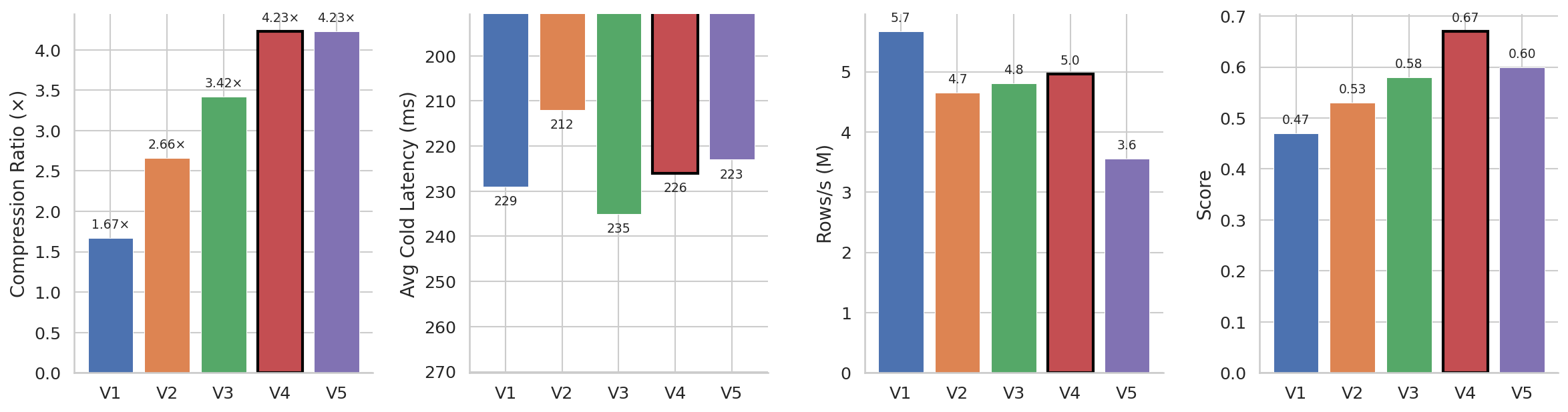
And as a decision tree:
Is your column a sorted timestamp?
  → Yes: DoubleDelta + ZSTD(3)                    [872× on sorted 1s intervals]
  → No: Is it a monotone counter?
    → Yes: Delta(8) + ZSTD(3)                      [843× on strictly monotone]
    → No: Is it a Float?
      → Smooth/slowly changing?  → Gorilla(8) + LZ4   [up to 45× on monotone floats]
      → Noisy/random?           → LZ4 default         [Gorilla hurts here]
    → String/LowCardinality?    → ZSTD(3)             [867–908×]
The takeaways I’d actually carry into production:
- Per-column codec choice is where the value is. V1 to V4 is 1.67× to 4.23×, and that comes from DoubleDelta and Delta, not from ZSTD.
- Skip ZSTD(9). On this data it compressed nothing extra and cost 28% ingest.
- Don’t put Gorilla on noisy floats. Measure first.
- Measure on your own data. My 800×+ ratios need perfectly regular intervals. Real metrics with variable scrape intervals will land somewhere between 10× and 100× on timestamps. Still great, just not 872×.
Limitations
Honest list, so you can judge how far these numbers carry:
- Synthetic, perfectly regular data. Real metrics compress less.
- Everything fits in RAM, single merged part, single-threaded queries. Production has many parts, concurrent load, and data bigger than memory. Each of these shifts the trade-offs, mostly in favor of better compression.
- Fixed query order, no randomization. Warm runs could carry cache effects between queries.
- I profiled decompression CPU for one query only (Q05). The explanation fits the other results but isn’t individually proven.
- FPC codec not tested. It targets floats and might beat both LZ4 and Gorilla on the noisy value column.
References
- Pelkonen, T., et al. “Gorilla: A Fast, Scalable, In-Memory Time Series Database.” VLDB 2015. PDF
- ClickHouse Compression Documentation
- Optimize Codecs & Schema (ClickHouse Blog)
- Altinity: New Encodings to Improve ClickHouse (2019)
Tested on ClickHouse 25.11.3.54, Hetzner CX53 (16 vCPU, 32 GB RAM, NVMe SSD). Raw data, scripts and plots: github.com/comino/blog-experiments.