ClickHouse Projections vs Materialized Views: A Practical Benchmark
Projections and materialized views benchmarked on 200M rows of web analytics data in ClickHouse: query speedup, storage and ingest cost, and the unmerged-parts case where both are slower than the base table.
- clickhouse
- performance
- data-modeling
- projections
- materialized-views
TLDR
- On 200M rows, aggregating projections and materialized views cut the tested cold aggregation from 470 ms to about 50 ms, with roughly 8% extra storage.
- Ingest throughput fell by 69–73% in the measured configurations. With merges stopped, both approaches became slower than the base table.
- Start with the base table, then choose projections for transparent SQL or materialized views for separate retention and cascading rollups. Keep background merges healthy.
I benchmarked ClickHouse projections against materialized views (MVs) on a 200M-row web analytics dataset: query latency, storage overhead, and ingest cost. I also tested what happens when background merges fall behind, and that turned out to be the most interesting result.
All data, scripts and plots: comino/blog-experiments. Numbers are median ± IQR over 10 runs.
The Difference in 30 Seconds
Projections live inside the table: an alternative sort order or a pre-aggregation stored per part. The optimizer picks them automatically, queries stay plain SQL. But it only picks them when GROUP BY and aggregation functions match exactly.
Materialized views write into a separate target table on every INSERT. You get full control over schema, engine and TTL, but queries against the target need -Merge() combinator functions like countMerge() and avgMerge().
Both store partial aggregate states that ClickHouse merges in the background. That shared mechanism is exactly why both fall over when merging lags, as you’ll see below.
Setup
- Server: Hetzner CX53 with 16 vCPU (AMD EPYC), 32 GB RAM, NVMe SSD
- ClickHouse: 25.11.3.54 (the multi-part experiment ran later on 26.1.2)
- Dataset: 200M synthetic web analytics rows (110M for the multi-part experiment)
- Cold runs: all ClickHouse and OS caches dropped before each measurement
- Data fits in RAM, so “cold” means NVMe re-read, not sustained disk I/O
Data Generation
INSERT INTO exp02_projections.web_analytics_base
SELECT
    toDateTime('2024-01-01') + rand(number) % (365 * 86400) AS timestamp,
    rand(number + 1) AS user_id,
    concat('/page/', toString(rand(number + 2) % 1000)) AS page,
    rand(number + 3) % 10000 AS duration_ms,
    ['US','UK','DE','FR','JP','CN','BR','IN','CA','AU','MX','KR','IT','ES','NL',
     'SE','NO','DK','FI','PL','CZ','AT','CH','BE','PT','IE','RU','TR','ZA','EG',
     'NG','KE','AR','CL','CO','PE','TH','VN','PH','MY','SG','ID','TW','HK','NZ',
     'IL','SA','AE','QA','UA'][1 + rand(number + 4) % 50] AS country,
    ['desktop', 'mobile', 'tablet'][1 + rand(number + 5) % 3] AS device_type
FROM numbers(200000000);
Timestamps span exactly one year (8,760 distinct hours), pages take 1,000 distinct values. That means the pre-aggregated key space is 1,000 × 8,760 = 8.76M (page, hour) combinations. This number shows up again and again below.
All tables use ORDER BY (page, timestamp). After insert, OPTIMIZE TABLE … FINAL merged each table into a single part (except in the multi-part experiment).
The Contenders
Base table, no tricks:
CREATE TABLE web_analytics_base (
    timestamp DateTime,
    user_id UInt32,
    page LowCardinality(String),
    duration_ms UInt32,
    country LowCardinality(String),
    device_type LowCardinality(String)
) ENGINE = MergeTree()
ORDER BY (page, timestamp);
Projection table: same schema plus two projections. One re-sorts the full data by country, one pre-aggregates hourly stats:
CREATE TABLE web_analytics_proj (
    -- ... same 6 columns ...
    PROJECTION proj_country_time (
        SELECT * ORDER BY country, timestamp
    ),
    PROJECTION proj_hourly_stats (
        SELECT page,
               toStartOfHour(timestamp) AS hour,
               count() AS hits,
               avg(duration_ms) AS avg_duration,
               sum(duration_ms) AS sum_duration
        GROUP BY page, hour
    )
) ENGINE = MergeTree()
ORDER BY (page, timestamp);MV: a target table with aggregate-state columns, fed by a materialized view:
CREATE TABLE hourly_stats_mv_target (
    page LowCardinality(String),
    hour DateTime,
    hits AggregateFunction(count, UInt64),
    avg_duration AggregateFunction(avg, UInt32),
    sum_duration AggregateFunction(sum, UInt32)
) ENGINE = AggregatingMergeTree()
ORDER BY (page, hour);

CREATE MATERIALIZED VIEW hourly_stats_mv
TO hourly_stats_mv_target AS
SELECT
    page,
    toStartOfHour(timestamp) AS hour,
    countState() AS hits,
    avgState(duration_ms) AS avg_duration,
    sumState(duration_ms) AS sum_duration
FROM web_analytics_mv_source
GROUP BY page, hour;
Note the -State functions. They store intermediate aggregation states, not final values. Reading them back requires the matching -Merge() functions.
Storage
| Configuration | Compressed | Overhead vs Base |
|---|---|---|
| Base only | 1.34 GB | baseline |
| Base + aggregating projection | 1.45 GB | +8% |
| MV source + MV target | 1.45 GB | +8% |
| Base + both projections (re-sort + agg) | 3.07 GB | +129% |
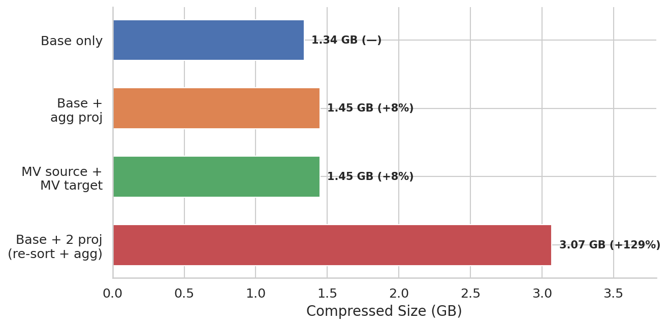
The aggregating projection and the MV target cost the same: ~108 MB for 8.76M pre-aggregated rows. The +129% case is the re-sort projection proj_country_time: it stores a complete second copy of all six columns, sorted differently. Know that before you add one.
Query Benchmark
Three queries against the 200M-row tables:
-- Q1: Point lookup (one page, one day)
SELECT count(), avg(duration_ms)
FROM web_analytics_base          -- or web_analytics_proj
WHERE page = '/page/0'
  AND timestamp BETWEEN '2024-01-15' AND '2024-01-16';

-- Q2: Country filter (one month). Country is not in the base sort key.
SELECT count(), avg(duration_ms)
FROM web_analytics_base          -- or web_analytics_proj
WHERE country = 'US'
  AND timestamp BETWEEN '2024-01-01' AND '2024-02-01';

-- Q3: Full aggregation (top pages by avg duration)
SELECT page, avg(duration_ms) AS avg_d
FROM web_analytics_base          -- or web_analytics_proj
GROUP BY page ORDER BY avg_d DESC LIMIT 10;

-- Q3 against the MV target needs -Merge():
SELECT page, avgMerge(avg_duration) AS avg_d
FROM hourly_stats_mv_target
GROUP BY page ORDER BY avg_d DESC LIMIT 10;
Results (median ± IQR, ms, n=10):
| Query | Base | Projection | MV Target | Notes |
|---|---|---|---|---|
| Q1 cold | 16 ± 4 | 18 ± 2 | 12 ± 1 | MV reads a smaller table |
| Q1 warm | 5 ± 0 | 7 ± 0 | 5 ± 0 | all tied |
| Q2 cold | 26 ± 1 | 23 ± 2 | n/a | re-sort projection helps a little |
| Q2 warm | 9 ± 1 | 11 ± 2 | n/a | no MV for country queries |
| Q3 cold | 470 ± 20 | 50 ± 2 | 49 ± 4 | 9.4× faster |
| Q3 warm | 178 ± 5 | 23 ± 1 | 23 ± 1 | both pre-agg tied |
What this says:
- Q1: the base
ORDER BY (page, timestamp)already handles point lookups well. Nothing to win here.EXPLAINconfirms the optimizer doesn’t even use a projection for this query. - Q2: the re-sort projection saves 3 ms cold. That’s what +129% storage buys on this query mix.
- Q3 is the whole story: instead of scanning 200M rows, both pre-aggregation approaches read the 8.76M-row summary. 470 ms becomes 50 ms.
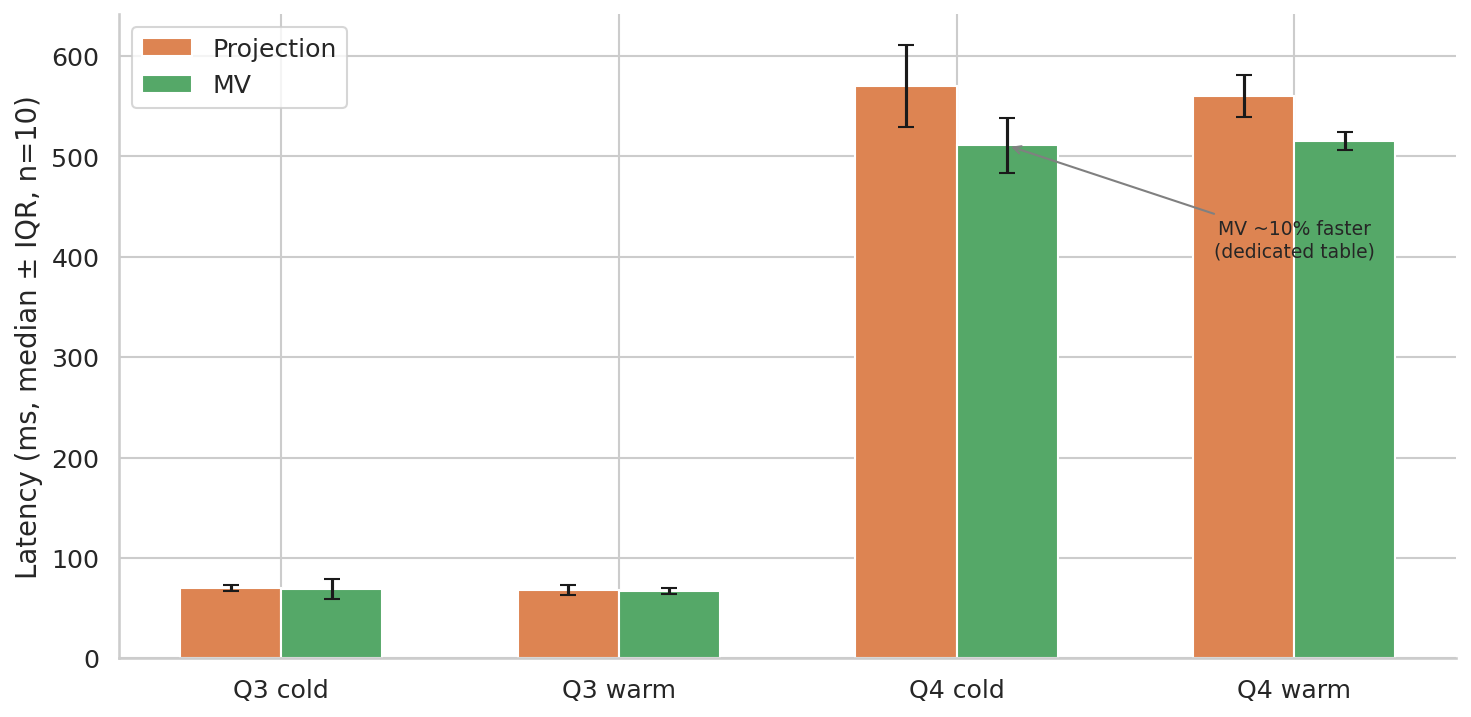
For a clean head-to-head I also ran an aggregating projection against an MV on two more query shapes (n=10): filtering one page is a tie (70 vs 69 ms cold), and a full scan across all pages has the MV ~10% ahead (511 vs 570 ms cold). Its dedicated AggregatingMergeTree table has a small edge over the projection, which shares storage with the base table.
What the Optimizer Actually Picks
Projections only fire when the query matches. I tested 8 patterns against the projection table:
| Query Pattern | Projection Used? | Why |
|---|---|---|
Point lookup (WHERE page=… AND ts=…) | ❌ | base sort key already optimal |
| Month rollup for one page | ❌ | page is the first sort key column |
| Country filter | ✅ re-sort | country not in base sort key |
| Country + time range | ✅ re-sort | both in projection sort key |
| Top-K by avg duration | ✅ aggregating | matches GROUP BY + aggregation |
| Top-K with HAVING | ✅ aggregating | still matches |
uniqExact(user_id) | ❌ | no projection covers user_id |
| Multi-dimension GROUP BY | ❌ | no matching projection |
A sum() query will not use a projection that stores avg(). An extra GROUP BY column breaks the match. Always check with EXPLAIN indexes=1 instead of assuming.
When Does Pre-Aggregation Pay Off?
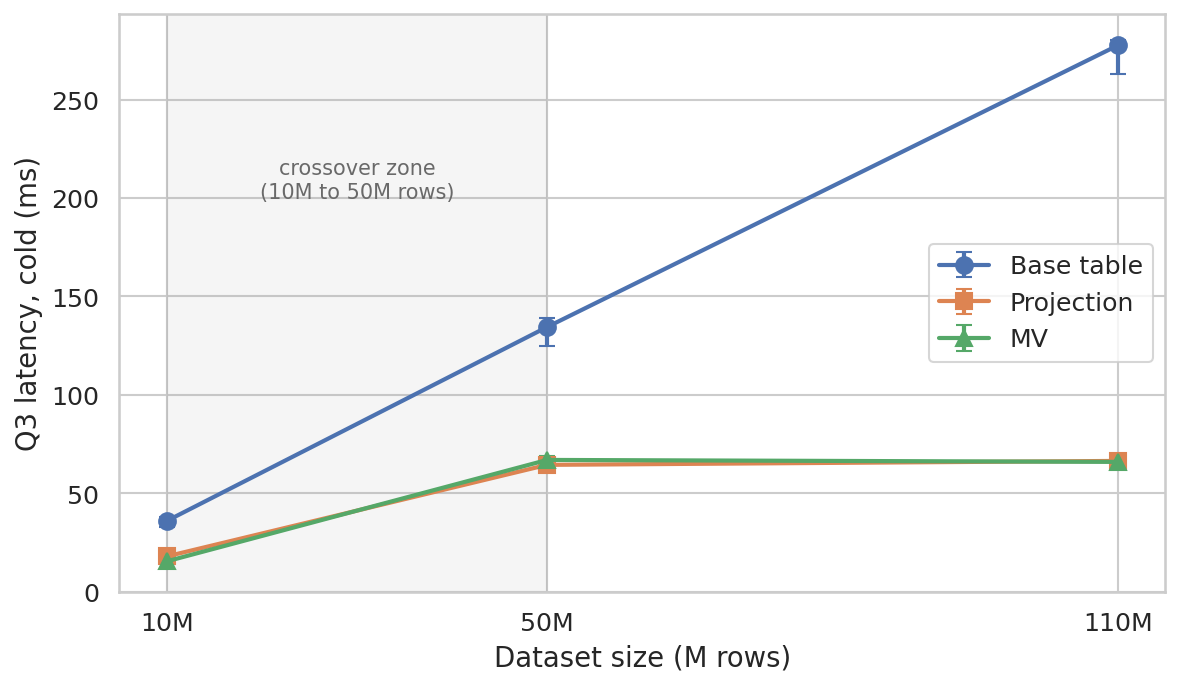
Same aggregation query (Q3) at three dataset sizes, single merged part, cold:
| Size | Base | Projection | MV | Speedup |
|---|---|---|---|---|
| 10M | 36 ± 3 ms | 18 ± 1 ms | 16 ± 1 ms | 2.0× |
| 50M | 134 ± 7 ms | 64 ± 3 ms | 67 ± 4 ms | 2.1× |
| 110M | 278 ± 9 ms | 66 ± 2 ms | 66 ± 2 ms | 4.2× |
At 10M rows the base scan takes 36 ms. Nobody needs to optimize that. The point where pre-aggregation starts to matter is somewhere between 10M and 50M rows for this query on this hardware.
The mechanism behind the growing speedup: the base scan grows linearly with table size, but the pre-aggregated summary is capped by its key space (8.76M rows, no matter how big the base table gets). The bigger the table, the bigger the win.
The Multi-Part Reality Check
Everything above used OPTIMIZE FINAL: one merged part, the best case. Production doesn’t look like that. Data streams in, parts pile up, and background merges have to catch up. So I built the bad case deliberately: 110M rows inserted in 11 batches with background merges stopped, leaving 55 unmerged parts.
The state before merging, from system.parts:
| Table | Parts | Rows | Disk |
|---|---|---|---|
| base | 55 | 110M | 1.31 GiB |
| projection table | 55 | 110M | 2.38 GiB |
| MV target | 110 | 98.3M | 1.07 GiB |
The MV target should have 8.76M rows. It has 98.3M, eleven times too many, because every unmerged part carries its own partial aggregates for the same (page, hour) keys.
Same aggregation query as before, on this state:
| State | Base | Projection | MV |
|---|---|---|---|
| 55 parts, cold | 270 ± 11 | 415 ± 20 | 470 ± 14 |
| 55 parts, warm | 108 ± 7 | 251 ± 19 | 252 ± 11 |
| merged, cold | 278 ± 17 | 66 ± 3 | 66 ± 4 |
| merged, warm | 96 ± 11 | 38 ± 2 | 39 ± 5 |
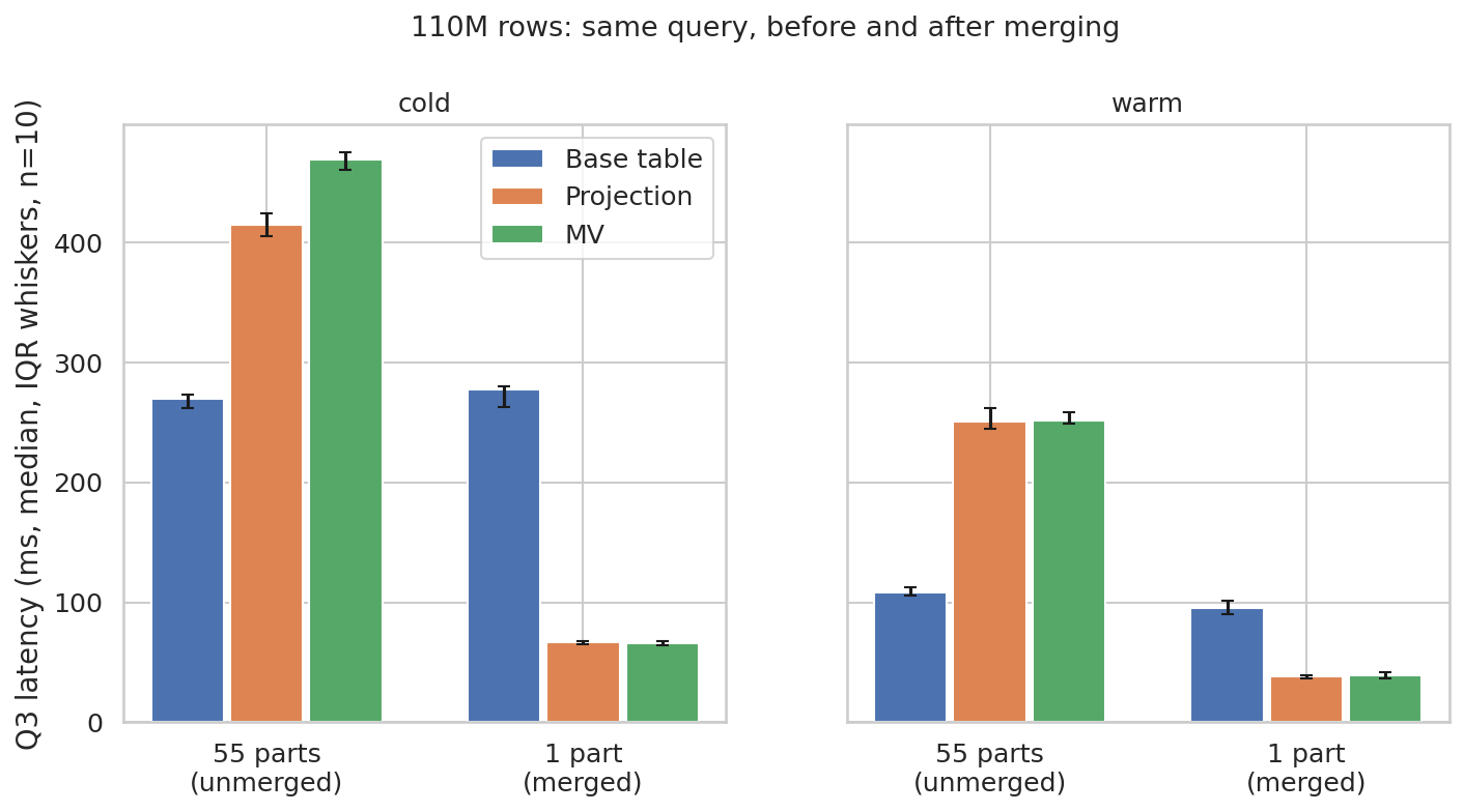
With 55 unmerged parts, the base table wins. The projection and MV queries had to read 98M rows of aggregate-state data, which is wider and more expensive per row than the base table’s plain integers. After OPTIMIZE FINAL, the MV target collapsed from 98.3M to 8.76M rows and both approaches delivered their 4.2× speedup.
What I take from this:
- Merging is a prerequisite, not a cleanup step. Unmerged projections and MVs can actively hurt.
- The MV target row count is your canary.
SELECT count() FROM mv_targetshould be close to your key-space size. Mine was 11× over. - High ingest with lagging merges is the danger zone. My 55-part state is an extreme; a production burst might create 5–20 parts with proportionally milder damage. But the direction is the same.
Ingest Cost
Ingest throughput, fresh tables, rand()-generated rows, n=10:
| Variant | 1M batch (rows/s) | 10M batch (rows/s) | vs Base (10M) |
|---|---|---|---|
| Base | 2,540K ± 151K | 3,000K ± 37K | baseline |
| Projection | 732K ± 31K | 820K ± 21K | −73% |
| MV | 672K ± 15K | 931K ± 18K | −69% |
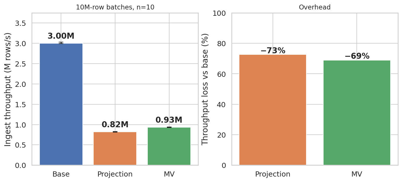
That is a lot. Both approaches compute aggregations on every insert, and it shows.
The absolute overhead depends on how you measure: in a second test that copied rows from an existing table instead of generating them (n=5), the projection cost 49% and the MV 30%. The ordering was the same in both tests: the MV is consistently the cheaper of the two on ingest, because it writes its aggregates to a separate table instead of computing them inside every part of the base table.
If ingest is your bottleneck, look at Refreshable Materialized Views (ClickHouse 23.12+): they recompute periodically instead of on every insert, trading freshness for write throughput. I didn’t benchmark them here.
Which One?
| Scenario | Recommendation |
|---|---|
| Dashboard aggregations, known query patterns | Either. Pick by ingest tolerance and syntax preference |
| Ad-hoc queries on a second sort dimension | Projection (re-sort), if the +100% storage is acceptable |
| Ingest-sensitive workload | MV, or Refreshable MV |
| Multi-level rollups (hourly → daily → monthly) | MV. Projections can’t cascade |
| Separate retention/TTL for aggregates | MV. Projections share the base table’s TTL |
| Small table (< a few 10M rows) | Neither. The scan is already fast |
| Minimal operational surface | Projection. No extra tables, plain SQL |
My default: start with the base table. When a specific aggregation query gets too slow, add an aggregating projection first, because it’s transparent to every query and every team member. Move to an MV when you need cascading, separate TTL, or cheaper ingest.
And whichever you pick: watch your parts. An unmerged MV target with 98M rows instead of 8.76M is not an optimization, it’s a regression.
Do you need an alternative sort order?
  → Yes: Re-sort projection (costs a full data copy)
  → No: Do you need pre-aggregation at all?  (< ~50M rows: probably not)
    → Ingest-critical, cascading rollups, or own TTL?
      → Yes: Materialized View (requires -Merge() syntax)
      → No:  Aggregating projection (transparent SQL)

Either way: monitor system.parts and keep background merges healthy.
Limitations
- Synthetic uniform data. Real traffic has power-law pages and geographic clustering. The 8.76M-key saturation behavior depends on my uniform distribution.
- Data fits in RAM. With data well beyond memory, pre-aggregation’s I/O advantage grows.
- The 55-part state is artificial. I stopped background merges to build it. It shows the mechanism, not a typical magnitude. The multi-part run also used a newer ClickHouse (26.1.2); the effect follows from the MergeTree architecture, not the version.
- Single writer. Concurrent inserts interact with merge scheduling in ways I didn’t measure.
- Refreshable MVs and MV chaining untested. Both would matter in a real decision.
- Projection operational caveats not explored: adding a projection later requires a full
MATERIALIZE PROJECTIONrescan, and projections share the base table’s TTL and partition lifecycle.
References
- Projections vs Materialized Views (ClickHouse Docs)
- Projections Deep Dive (ClickHouse Docs)
- Altinity: Projection Examples
- Refreshable Materialized Views (ClickHouse Docs)
Tested on ClickHouse 25.11.3.54 / 26.1.2, Hetzner CX53 (16 vCPU, 32 GB RAM, NVMe SSD). Raw data, scripts and plots: github.com/comino/blog-experiments.